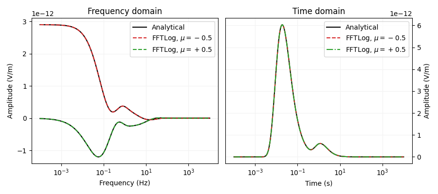
Geophysical Electromagnetic modelling

In this example we use pyfftlog to obtain time-domain EM data from frequency-domain data and vice versa. We do this by using analytical halfspace solution in both domains, and comparing the transformed responses to the true result. The analytical halfspace solutions are computed using empymod (see https://empymod.github.io).

import empymod
import pyfftlog
import numpy as np
import matplotlib.pyplot as plt
from scipy.interpolate import InterpolatedUnivariateSpline as iuSpline

Model and Survey parameters

# Impulse response (in the time domain)
signal = 0

# x-directed electric source and receiver point-dipoles
ab = 11

# We use the same range of times (s) and frequencies (Hz)
ftpts = np.logspace(-4, 4, 301)

# Source and receiver
src = [0, 0, 100]     # At the origin, 100 m below surface
rec = [6000, 0, 200]  # At an inline offset of 6 km, 200 m below surface

# Resistivity
depth = [0]      # Interface at z = 0, default for empymod.analytical
res = [2e14, 1]  # Horizontal resistivity [air, subsurface]
aniso = [1, 2]   # Anisotropy [air, subsurface]

# Collect parameters
analytical = {
    'src': src,
    'rec': rec,
    'res': res[1],
    'aniso': aniso[1],
    'solution': 'dhs',  # Diffusive half-space solution
    'verb': 2,
    'ab': ab,
}

dipole = {
    'src': src,
    'rec': rec,
    'depth': depth,
    'res': res,
    'aniso': aniso,
    'ht': 'dlf',
    'verb': 2,
    'ab': ab,
}

Analytical solutions

# Frequency Domain
f_ana = empymod.analytical(**analytical, freqtime=ftpts)

# Time Domain
t_ana = empymod.analytical(**analytical, freqtime=ftpts, signal=signal)

Out:

:: empymod END; runtime = 0:00:00.002148 ::


:: empymod END; runtime = 0:00:00.001233 ::

FFTLog

# FFTLog parameters
pts_per_dec = 5    # Increase if not precise enough
add_dec = [-2, 2]  # e.g. [-2, 2] to add 2 decades on each side
q = 0              # -1 - +1; can improve results

# Compute minimum and maximum required inputs
rmin = np.log10(1/ftpts.max()) + add_dec[0]
rmax = np.log10(1/ftpts.min()) + add_dec[1]
n = np.int(rmax - rmin)*pts_per_dec

# Pre-allocate output
f_resp = np.zeros(ftpts.shape, dtype=complex)

# Loop over Sine, Cosine transform.
for mu in [0.5, -0.5]:

    # Central point log10(r_c) of periodic interval
    logrc = (rmin + rmax)/2

    # Central index (1/2 integral if n is even)
    nc = (n + 1)/2.

    # Log spacing of points
    dlogr = (rmax - rmin)/n
    dlnr = dlogr*np.log(10.)

    # Compute required input x-values
    pts_req = 10**(logrc + (np.arange(1, n+1) - nc)*dlogr)/2/np.pi

    # Initialize FFTLog
    kr, xsave = pyfftlog.fhti(n, mu, dlnr, q, kr=1, kropt=1)

    # Compute pts_out with adjusted kr
    logkc = np.log10(kr) - logrc
    pts_out = 10**(logkc + (np.arange(1, n+1) - nc)*dlogr)

    # rk = r_c/k_r; adjust for Fourier transform scaling
    rk = 10**(logrc - logkc)*np.pi/2

    # Compute required times/frequencies with the analytical solution
    t2f_t_resp = empymod.analytical(**analytical, freqtime=pts_req,
                                    signal=signal)
    f2t_f_resp = empymod.analytical(**analytical, freqtime=pts_req)

    # Carry out FFTLog
    t2f_f_coarse = pyfftlog.fftl(t2f_t_resp, xsave.copy(), rk, 1)
    if mu > 0:
        f2t_t_coarse = pyfftlog.fftl(f2t_f_resp.imag, xsave.copy(), rk, 1)
    else:
        f2t_t_coarse = pyfftlog.fftl(f2t_f_resp.real, xsave.copy(), rk, 1)

    # Interpolate for required frequencies/times
    t2f_f_spline = iuSpline(np.log(pts_out), t2f_f_coarse)
    f2t_t_spline = iuSpline(np.log(pts_out), f2t_t_coarse)

    if mu > 0:
        f_resp += -1j*t2f_f_spline(np.log(ftpts))/np.pi/2
        t_resp_sin = -f2t_t_spline(np.log(ftpts))/np.pi*2
    else:
        f_resp += t2f_f_spline(np.log(ftpts))/np.pi/2
        t_resp_cos = f2t_t_spline(np.log(ftpts))/np.pi*2

Out:

/home/docs/checkouts/readthedocs.org/user_builds/pyfftlog/checkouts/latest/examples/geophysical_em.py:86: DeprecationWarning: `np.int` is a deprecated alias for the builtin `int`. To silence this warning, use `int` by itself. Doing this will not modify any behavior and is safe. When replacing `np.int`, you may wish to use e.g. `np.int64` or `np.int32` to specify the precision. If you wish to review your current use, check the release note link for additional information.
Deprecated in NumPy 1.20; for more details and guidance: https://numpy.org/devdocs/release/1.20.0-notes.html#deprecations
  n = np.int(rmax - rmin)*pts_per_dec

:: empymod END; runtime = 0:00:00.000758 ::


:: empymod END; runtime = 0:00:00.001016 ::


:: empymod END; runtime = 0:00:00.000837 ::


:: empymod END; runtime = 0:00:00.000978 ::

Comparison

fig, (ax0, ax1) = plt.subplots(1, 2, figsize=(9, 4))

# TIME DOMAIN
ax0.set_title(r'Frequency domain')
ax0.set_xlabel('Frequency (Hz)')
ax0.set_ylabel('Amplitude (V/m)')
ax0.semilogx(ftpts, f_ana.real, 'k-', label='Analytical')
ax0.semilogx(ftpts, f_ana.imag, 'k-')
ax0.semilogx(ftpts, f_resp.real, 'C3--', label=r'FFTLog, $\mu=-0.5$')
ax0.semilogx(ftpts, f_resp.imag, 'C2--', label=r'FFTLog, $\mu=+0.5$')
ax0.legend(loc='best')
ax0.grid(which='both', c='.95')

# TIME DOMAIN
ax1.set_title(r'Time domain')
ax1.set_xlabel('Time (s)')
ax1.set_ylabel('Amplitude (V/m)')
ax1.semilogx(ftpts, t_ana, 'k', label='Analytical')
ax1.semilogx(ftpts, t_resp_cos, 'C3--', label=r'FFTLog, $\mu=-0.5$')
ax1.semilogx(ftpts, t_resp_sin, 'C2-.', label=r'FFTLog, $\mu=+0.5$')
ax1.legend(loc='best')
ax1.yaxis.set_label_position("right")
ax1.yaxis.tick_right()
ax1.grid(which='both', c='.95')

fig.tight_layout()
fig.show()