Sine Transform

Contributed by @ShazAlvi.

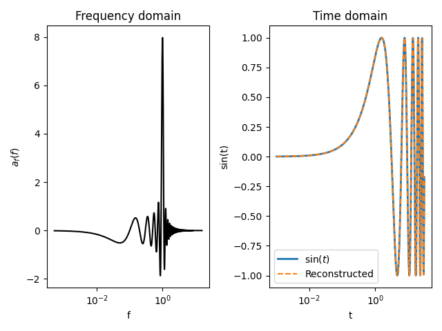
This is a simple test program to illustrate how the sine (or cosine as it works basically the same way ) Fourier transform works using FFTLog. The test provides as input as sine function and performs the sine Fourier transform. The input function is then recovered by performing an inverse Fourier transform. The inverse is performed using the following integral,

(1)\[F(t) = \sqrt{\frac{\pi}{2}}\int^\infty_0 A(f)\ \sin(ft) \ \text{d}f \ .\]

import pyfftlog
import numpy as np
import scipy.integrate
import matplotlib.pyplot as plt

Define the parameters you wish to use

The presets are the Reasonable choices of parameters from fftlogtest.f.

# Range of periodic interval
logtmin = -3
# logtmax = 0.798 #2pi
# 5(2pi) #Longer range in r gives you a better reconstruction. 10\pi will give
# you a better reconstruction than 2\pi.
logtmax = 1.497
# Number of points (Max 4096)
# 1000 points give you a fairly smooth distribution of af in frequency, f.
# However you can get a good, working fit for 300 points as well.
n = 1000

# Order mu of Bessel function
mu = 0.5  # Choose -0.5 for cosine fourier transform

# Bias exponent: q = 0 is unbiased
# The unbiased transforms give better results as far as I checked.
q = 0
# Sensible approximate choice of f_c t_c
# The output and the reconstruction is sensitive to the choice of this value
# This value is found by trial and error. In this example, the input function
# is a simple sine function which is not smooth in frequency space (as it
# only has one frequency) because of this reason a better value of this
# quantity is not found by the function fhti. For functions smooth
# in both time and frequency domain, the fhti should return the best
# value of the f_c t_c.

ft = 0.016

# Tell fhti to change ft to low-ringing value
# WARNING: kropt = 3 will fail, as interaction is not supported
ftopt = 1

# Forward transform (changed from dir to tdir, as dir is a python fct)
tdir = 1

Computation related to the logarithmic spacing

# Central point log10(t_c) of periodic interval
logtc = (logtmin + logtmax)/2

print(f"Central point of periodic interval at log10(t_c) = {logtc}")

# Central index (1/2 integral if n is even)
nc = (n + 1)/2.0

# Log-spacing of points
dlogt = (logtmax - logtmin)/n

dlnr = dlogt*np.log(10.0)

Out:

Central point of periodic interval at log10(t_c) = -0.7515

Compute input function: \(\sin(t)\)

t = 10**(logtc + (np.arange(1, n+1) - nc)*dlogt)
a_t = np.sin(t)

Initialize FFTLog transform - note fhti resets ft

ft, xsave = pyfftlog.fhti(n, mu, dlnr, q, ft, ftopt)

Call pyfftlog.fhtl

logfc = np.log10(ft) - logtc

# Fourier sine Transform
a_f = pyfftlog.fftl(a_t.copy(), xsave, np.sqrt(2/np.pi), tdir)
# Notice that np.sqrt(2/np.pi) is the normalization factor for the transform
# Reconstruct the input function by taking the inverse fourier transform as
# given in the description
f = 10**(logfc + (np.arange(1, n+1) - nc)*dlogt)
# Array to store the reconstructed function for each value of t
Recon_Fun = np.zeros((len(t)))
for i in range(len(t)):
    Recon_Fun[i] = (np.sqrt(2/np.pi)**-1) * \
       scipy.integrate.trapz(f, a_f*np.sin(t[i]*f))

# Plotting the input function and the reconstructed input function and also
# the distribution of the a(f) vs f.
plt.figure()

ax1 = plt.subplot(121)
plt.title(r'Frequency domain')
plt.xlabel('f')
plt.ylabel(r'$a_f(f)$')
plt.semilogx(f, a_f, 'k')

ax2 = plt.subplot(122)
plt.title('Time domain')
plt.xlabel("t")
plt.ylabel("sin(t)")
plt.semilogx(t, a_t, lw=2, label=r'$\sin(t)$')
plt.semilogx(t, -Recon_Fun, '--', label='Reconstructed')
plt.legend()

plt.tight_layout()
plt.show()