Note
Go to the end to download the full example code.
FFTLog-Test
This example is a translation of fftlogtest.f from the Fortran package FFTLog, which was presented in Appendix B of [Hami00] and published at https://jila.colorado.edu/~ajsh/FFTLog. It serves as an example for the python package pyfftlog (which is a Python version of FFTLog), in the same manner as the original file fftlogtest.f serves as an example for Fortran package FFTLog.
What follows is the original documentation from the file `fftlogtest.f`:
This is fftlogtest.f
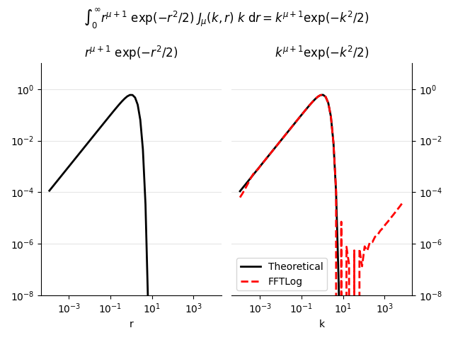
This is a simple test program to illustrate how FFTLog works. The test transform is:
Disclaimer
FFTLog does NOT claim to provide the most accurate possible solution of the continuous transform (which is the stated aim of some other codes). Rather, FFTLog claims to solve the exact discrete transform of a logarithmically-spaced periodic sequence. If the periodic interval is wide enough, the resolution high enough, and the function well enough behaved outside the periodic interval, then FFTLog may yield a satisfactory approximation to the continuous transform.
Observe:
How the result improves as the periodic interval is enlarged. With the normal FFT, one is not used to ranges orders of magnitude wide, but this is how FFTLog prefers it.
How the result improves as the resolution is increased. Because the function is rather smooth, modest resolution actually works quite well here.
That the central part of the transform is more reliable than the outer parts. Experience suggests that a good general strategy is to double the periodic interval over which the input function is defined, and then to discard the outer half of the transform.
That the best bias exponent seems to be \(q = 0\).
That for the critical index \(\mu = -1\), the result seems to be offset by a constant from the ‘correct’ answer.
That the result grows progressively worse as mu decreases below -1.
The analytic integral above fails for \(\mu \le -1\), but FFTLog still returns answers. Namely, FFTLog returns the analytic continuation of the discrete transform. Because of ambiguity in the path of integration around poles, this analytic continuation is liable to differ, for \(\mu \le -1\), by a constant from the ‘correct’ continuation given by the above equation.
FFTLog begins to have serious difficulties with aliasing as \(\mu\) decreases below \(-1\), because then \(r^{\mu+1} \exp(-r^2/2)\) is far from resembling a periodic function. You might have thought that it would help to introduce a bias exponent \(q = \mu\), or perhaps \(q = \mu+1\), or more, to make the function \(a(r) = A(r) r^{-q}\) input to fhtq more nearly periodic. In practice a nonzero \(q\) makes things worse.
A symmetry argument lends support to the notion that the best exponent here should be \(q = 0,\) as empirically appears to be true. The symmetry argument is that the function \(r^{\mu+1} \exp(-r^2/2)\) happens to be the same as its transform \(k^{\mu+1} \exp(-k^2/2)\). If the best bias exponent were q in the forward transform, then the best exponent would be \(-q\) that in the backward transform; but the two transforms happen to be the same in this case, suggesting \(q = -q\), hence \(q = 0\).
This example illustrates that you cannot always tell just by looking at a function what the best bias exponent \(q\) should be. You also have to look at its transform. The best exponent \(q\) is, in a sense, the one that makes both the function and its transform look most nearly periodic.
import pyfftlog
import numpy as np
import matplotlib.pyplot as plt
Define the parameters you wish to use
The presets are the Reasonable choices of parameters from fftlogtest.f.
# Range of periodic interval
logrmin = -4
logrmax = 4

# Number of points (Max 4096)
n = 64

# Order mu of Bessel function
mu = 0

# Bias exponent: q = 0 is unbiased
q = 0

# Sensible approximate choice of k_c r_c
kr = 1

# Tell fhti to change kr to low-ringing value
# WARNING: kropt = 3 will fail, as interaction is not supported
kropt = 1

# Forward transform (changed from dir to tdir, as dir is a python fct)
tdir = 1
Compute input function: \(r^{\mu+1}\exp\left(-\frac{r^2}{2}\right)\)
Initialize FFTLog transform - note fhti resets kr
pyfftlog.fhti: new kr = 0.9535389675791917
Call pyfftlog.fht (or pyfftlog.fhtl)
Central point in k-space at log10(k_c) = -0.020661554260541743
Compute Output function: \(k^{\mu+1}\exp\left(-\frac{k^2}{2}\right)\)
Plot result
plt.figure()

# Input
ax1 = plt.subplot(121)
plt.title(r'$r^{\mu+1}\ \exp(-r^2/2)$')
plt.xlabel('r')

plt.loglog(r, ar, 'k', lw=2)

plt.grid(axis='y', c='0.9')

# Transformed result
ax2 = plt.subplot(122, sharey=ax1)
plt.title(r'$k^{\mu+1} \exp(-k^2/2)$')
plt.xlabel('k')

plt.loglog(k, theo, 'k', lw=2, label='Theoretical')
plt.loglog(k, ak, 'r--', lw=2, label='FFTLog')

plt.legend()
plt.ylim([1e-8, 1e1])

ax2.yaxis.tick_right()
ax2.yaxis.set_label_position("right")
plt.grid(axis='y', c='0.9')

# Switch off spines
ax1.spines['top'].set_visible(False)
ax1.spines['right'].set_visible(False)
ax2.spines['top'].set_visible(False)
ax2.spines['left'].set_visible(False)
plt.tight_layout(rect=[0, 0, 1, .9])

# Main title
plt.suptitle(r"$\int_0^\infty r^{\mu+1}\ \exp(-r^2/2)\ J_\mu(k,r)\ " +
             r"k\ {\rm d}r = k^{\mu+1} \exp(-k^2/2)$", y=0.98)

plt.show()
Print values
           k                 a(k)       k^(mu+1) exp(-k^2/2)
----------------------------------------------------------------
      1.101130e-04       6.332603e-05       1.101130e-04
      1.468380e-04       9.168618e-05       1.468380e-04
      1.958116e-04       1.374282e-04       1.958116e-04
      2.611190e-04       2.131954e-04       2.611190e-04
      3.482078e-04       3.318802e-04       3.482077e-04
      4.643425e-04       4.923984e-04       4.643425e-04
      6.192107e-04       6.460278e-04       6.192106e-04
      8.257307e-04       7.968931e-04       8.257304e-04
      1.101130e-03       1.113736e-03       1.101129e-03
      1.468380e-03       1.464233e-03       1.468378e-03
      1.958116e-03       1.959475e-03       1.958112e-03
      2.611190e-03       2.610678e-03       2.611181e-03
      3.482078e-03       3.482260e-03       3.482056e-03
      4.643425e-03       4.643299e-03       4.643375e-03
      6.192107e-03       6.191999e-03       6.191988e-03
      8.257307e-03       8.257056e-03       8.257026e-03
      1.101130e-02       1.101057e-02       1.101063e-02
      1.468380e-02       1.468230e-02       1.468222e-02
      1.958116e-02       1.957729e-02       1.957741e-02
      2.611190e-02       2.610314e-02       2.610300e-02
      3.482078e-02       3.479950e-02       3.479967e-02
      4.643425e-02       4.638444e-02       4.638422e-02
      6.192107e-02       6.180220e-02       6.180247e-02
      8.257307e-02       8.229239e-02       8.229205e-02
      1.101130e-01       1.094470e-01       1.094474e-01
      1.468380e-01       1.452640e-01       1.452635e-01
      1.958116e-01       1.920928e-01       1.920934e-01
      2.611190e-01       2.523680e-01       2.523671e-01
      3.482078e-01       3.277241e-01       3.277250e-01
      4.643425e-01       4.168889e-01       4.168871e-01
      6.192107e-01       5.111853e-01       5.111866e-01
      8.257307e-01       5.871956e-01       5.871927e-01
      1.101130e+00       6.005500e-01       6.005516e-01
      1.468380e+00       4.996049e-01       4.996187e-01
      1.958116e+00       2.879340e-01       2.879045e-01
      2.611190e+00       8.632888e-02       8.634968e-02
      3.482078e+00       8.102022e-03       8.108819e-03
      4.643425e+00       1.180344e-04       9.656964e-05
      6.192107e+00      -1.553139e-05       2.923736e-08
      8.257307e+00       7.225353e-06       1.291402e-14
      1.101130e+01      -2.588950e-06       5.164519e-26
      1.468380e+01       7.719794e-07       2.222595e-46
      1.958116e+01       1.586977e-07       1.078537e-82
      2.611190e+01      -1.874092e-07      2.285953e-147
      3.482078e+01       5.576689e-07      1.793712e-262
      4.643425e+01      -1.317041e-07       0.000000e+00
      6.192107e+01       6.415736e-07       0.000000e+00
      8.257307e+01       1.351283e-07       0.000000e+00
      1.101130e+02       7.997181e-07       0.000000e+00
      1.468380e+02       5.394094e-07       0.000000e+00
      1.958116e+02       1.165867e-06       0.000000e+00
      2.611190e+02       1.176786e-06       0.000000e+00
      3.482078e+02       1.889416e-06       0.000000e+00
      4.643425e+02       2.248731e-06       0.000000e+00
      6.192107e+02       3.228937e-06       0.000000e+00
      8.257307e+02       4.113223e-06       0.000000e+00
      1.101130e+03       5.651921e-06       0.000000e+00
      1.468380e+03       7.408687e-06       0.000000e+00
      1.958116e+03       1.001142e-05       0.000000e+00
      2.611190e+03       1.330606e-05       0.000000e+00
      3.482078e+03       1.792186e-05       0.000000e+00
      4.643425e+03       2.410633e-05       0.000000e+00
      6.192107e+03       3.277422e-05       0.000000e+00
      8.257307e+03       4.510046e-05       0.000000e+00
Total running time of the script: (0 minutes 0.531 seconds)